
Routing Algorithms
Routing algorithms determine how a router gathers and reports reachability information, how it deals with topology changes, and how it determines the optimal route to a destination. Various types of routing algorithms exist, and each algorithm has a different impact on network and router resources. Routing algorithms use a variety of metrics that affect calculation of optimal routes. You can classify routing algorithms in the following major categories.
Static Routes and Dynamic Routing Protocols
Static routes are route table entries that you manually configure. These static routes do not change unless you reconfigure them. Static routes are simple to design and work well in environments where network traffic is relatively predictable and where network design is relatively simple.
Because static routing systems cannot react to network changes, you should not use them for large, constantly changing networks. Most routing protocols today use dynamic routing algorithms that adjust to changing network circumstances by analyzing incoming routing update messages. If the message indicates that a network change has occurred, the routing software recalculates routes and sends out new routing update messages. These messages permeate the network, triggering routers to rerun their algorithms and change their routing tables accordingly.
Interior and Exterior Gateway Protocols
You can separate networks into unique routing domains or autonomous systems. Routing protocols that route between autonomous systems are called exterior gateway protocols (EGPs) or interdomain protocols. The Border Gateway Protocol (BGP) is an example of an exterior gateway protocol (IGPs). Routing protocols used within an autonomous system are called interior gateway protocols or intradomain protocols. RIPv2, EIGRP, and OSPF are examples of interior gateway protocols.
Figure 6-2 shows various interior and exterior gateway protocols.
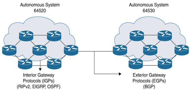
Figure 6-2 Interior and Exterior Gateway Protocols
Distance Vector and Link-State Protocols
Distance vector protocols use distance vector algorithms (also known as Bellman-Ford algorithms) that call for each router to send all or some portion of its routing table to its neighbors. Distance vector algorithms define routes by distance (for example, the number of hops to the destination) and direction (for example, the next-hop router). These routes are then broadcast to the directly connected neighbor routers. Each router uses these updates to verify and update the routing tables.
Figure 6-3 shows a routing table example for a distance vector protocol.
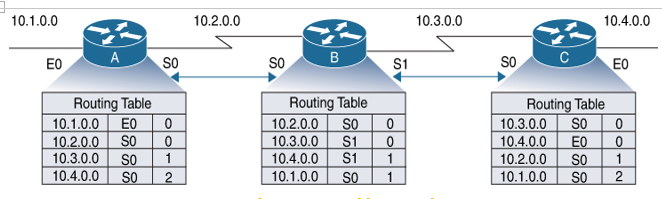
Figure 6-3 Distance Vector Protocol—Routing Table Example
To prevent routing loops, most distance vector algorithms use split horizon with poison reverse, which means that the routes learned from an interface are set as unreachable and advertised back along the interface that they were learned on during the next periodic update. This process prevents the router from seeing its own route updates coming back.
Distance vector algorithms send updates at fixed intervals but can also send updates in response to changes in route metric values. These triggered updates can speed up the route convergence time. The Routing Information Protocol (RIP) is a distance vector protocol.
Figure 6-4 illustrates a distance vector protocol update mechanism.
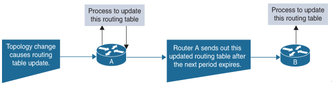
Figure 6-4 Distance Vector Protocol—Update Mechanism
The link-state protocols, also known as shortest path first (SPF), use the Dijkstra algorithm to find the shortest path between two nodes in the network. Each router shares information with neighboring routers and builds a link-state advertisement (LSA) that contains information about each link and directly connected neighbor routers. Each LSA has a sequence number. When a router receives an LSA and updates its link-state database, the LSA is flooded to all adjacent neighbors. If a router receives two LSAs with the same sequence number (from the same router), the router does not flood the last LSA it received to its neighbors because it wants to prevent an LSA update loop. Because the router floods the LSAs immediately after it receives them, the convergence time for link-state protocols is minimized.
Figure 6-5 illustrates the link-state protocol update and convergence mechanism.
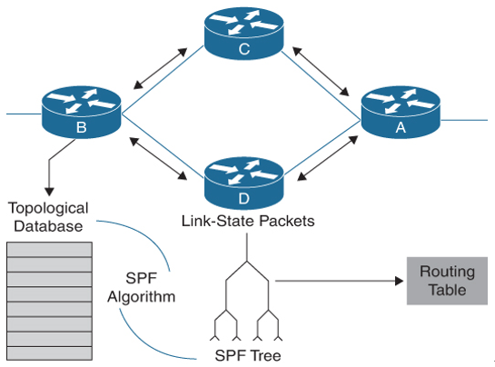
Figure 6-5 Link-State Protocol—Update and Convergence Mechanism
Discovering neighbors and establishing adjacency is an important part of a link-state protocol. Neighbors are discovered using special Hello packets that also serve as keepalive notifications to each neighbor router. Adjacency is the establishment of a common set of operating parameters for the link-state protocol between neighbor routers.
The LSAs received by a router are added to the router’s link-state database. Each entry consists of the following parameters:
- Router ID (for the router that originated the LSA)
- Neighbor ID
- Link cost
- Sequence number of the LSA
- Age of the LSA entry
The router runs the SPF algorithm on the link-state database, building the shortest path tree for that router. This SPF tree is used to populate the routing table. In link-state algorithms, each router builds a picture of the entire network in its routing tables. The link-state algorithms send small updates everywhere, while distance vector algorithms send larger updates only to neighboring routers. Because they converge more quickly, link-state algorithms are less likely to cause routing loops than distance vector algorithms. However, link-state algorithms require more CPU power and memory than distance vector algorithms, and they can be more expensive to implement and support. Link-state protocols are generally more scalable than distance vector protocols. OSPF is an example of a link-state protocol.
Table 6-2 compares a distance vector protocol with a link-state protocol.
Table 6-2 Distance Vector vs. Link-State Protocol
| Distance Vector Protocol | Link-State Protocol |
| Routers communicate with neighbor routers, advertising networks as a measure of distance and direction/vector. | Routers communicate with all other routers, exchanging link-state information to build a topology of the entire network. |
| Each router is aware only of its immediate neighbors. | Each router is aware of all other routers in the area. |
| Uses Bellman-Ford algorithm to calculate the shortest path. | Uses Dijkstra algorithm to calculate the shortest path. |
| Frequent updates of entire routing table. | Event-triggered partial updates. |
| Convergence is slow. | Convergence is fast. |
| Examples include RIPv2 and EIGRP. | Examples include OSPF and IS-IS. |